Deep Learning 101

Machine Learning

Neural Network

Posted at 2024/12/237 min to read

#Before we dive in...

Welcome to my post on Deep Learning. Here, I talk on Deep Learning in multiple parts. I hope you gain fundamental idea for computer science and statistics! I try to make content easy to read, but any comments are welcomed!

#Deep Learning

So Deep Learning refers to neural networks with multiple layers between input and output. Each of neurons enables complex data processing. Advantages Over Other Methods is layered structure excels in feature extraction and hierarchical processing, making it effective for image, speech, and similar data types. As we can see in nowadays, we got to see numbers of example AI model in image, speech, and similar data types.

Deep Learning algorithms allow efficient training of networks with many hidden layers. There are numbers of algorithms, with hundreds introduced annually. Every algorithm comprises three components:

Representation: The model's structure.
Evaluation: The method of measuring performance.
Optimization: The process of improving the model.

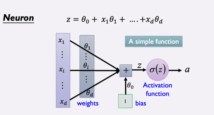
#Artificial Neuron

The Neuron Metaphor
In Machine learning and deep learning area, we got idea of neuron from brain cell. Neurons accept information from multiple inputs and transmit it to other neurons. Inputs are multiplied by weights/parameters. Apply a function to inputs at each node.

For example equation could be:
$z = \theta_0 + \theta_1 x_1 + \theta_2 x_2 + \dots + \theta_p x_p$

#Activation Functions

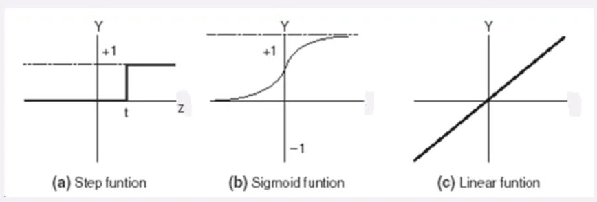
Activation functions determine the output of a neuron. They add non-linear properties, making the network capable of learning and representing complex relationships. We have couple famous activation functions. Here are just examples.

Sigmoid (logistic) function
The sigmoid function maps any real-valued number to a range between 0 and 1. It’s widely used for binary classification problems.

\sigma(z) = \frac{1}{1 + e^{-z}}

Hyperbolic tangent
The tanh function maps inputs to values between -1 and 1, making it zero-centered and often a better choice than the sigmoid function for certain applications.

\text{tanh}(z) = \frac{e^z - e^{-z}}{e^z + e^{-z}}

#Single Layer Neural Networks (NN)

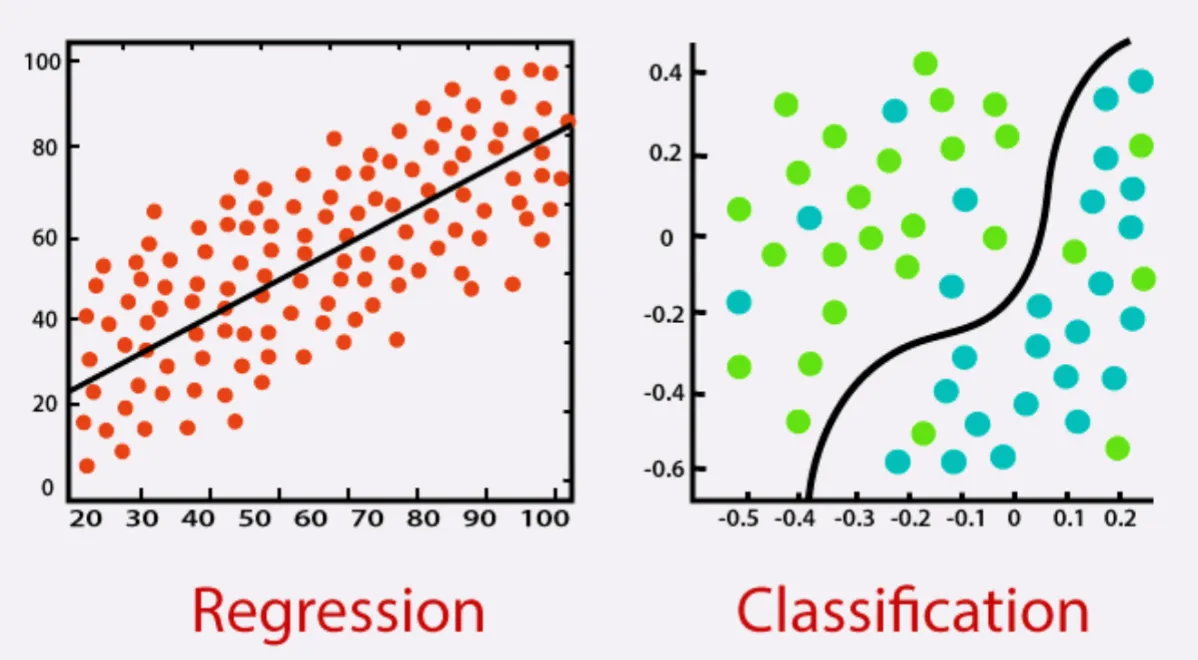
Linear Regression
A method to predict a dependent variable (y) based on one or more independent variables (x).

Least Squares Method
A method used in regression to minimize the difference between predicted and actual values.

Gradient Descent Algorithm
An iterative optimization technique used to minimize the cost function by updating model parameters (weights).

Linear Classification
A technique used to classify data points by drawing a straight line or hyperplane to separate classes.

Logistic Regression for Classification - A classification algorithm that maps input features to discrete outcomes (such as 0 or 1) using the logistic function.

For a point 𝑥 in feature space, project it onto 𝜃 to convert it into a real number 𝑧 in the range −∞ to +∞:. Map 𝑧 to the range 0 to 1 using the logistic (sigmoid) function:

$p = y(x) = \sigma(z) = \frac{1}{1 + e^{-z}}$

Overall, logistic regression maps a point in d-dimensional space to a value in the range 0 to 1.

#Combining Neurons

#Machine Learning ≈ Looking for a Function

Examples of functions in various applications:

Speech Recognition: $f(\text{input}) = \text{"How are you"}$
Image Recognition: $f(\text{image}) = \text{"Cat"}$
Playing Go: $f(\text{current board}) = \text{"5-5"} \ (\text{next move})$
Dialogue System: $f(\text{user input}) = \text{"Hello"} \ (\text{system response})$

#Three Steps for Deep Learning

Define a set of functions:
- Use a neural network.
Goodness of function:
- Evaluate the function's performance.
Pick the best function:
- Choose the function that performs the best.

#Step 1: Input Layer

The input layer has two inputs: ([0, 0]) as shown in the image.

#Step 2: First Hidden Layer

For each neuron in the first hidden layer, apply the formula. $z = \sum (\text{input} \times \text{weight}) + \text{bias}$ Then apply the activation function (typically the sigmoid function here).We will compute the outputs for each neuron in the hidden layer:

#Output Types:

The type of output in a machine learning model dictates the output layer and the cost function used. Common output types include:

Output Type	Output Distribution	Output Layer	Cost Function
Binary	Bernoulli	Sigmoid	Binary cross-entropy
Discrete	Multinoulli	Softmax	Discrete cross-entropy
Continuous	Gaussian	Linear	Gaussian cross-entropy or MSE
Continuous (Mixture of Gaussian)	Mixture Density	Mixture Density	Cross-entropy
Continuous (Arbitrary)	See advanced techniques such as GAN, VAE, FVBN	Varies	Various

#Softmax Layer

A softmax layer is commonly used as the output layer in classification tasks, especially when predicting probabilities for multiple discrete categories. It converts raw scores (logits) from the network into a probability distribution over the possible classes.

#Softmax Function

For a given set of scores ( z_1, z_2, z_3, \dots, z_n ), the softmax function normalizes them into probabilities:

y*j = \frac{e^{z_j}}{\sum*{i=1}^{n} e^{z_i}}

Where:

( y_j ) represents the probability for class ( j ).
( z_j ) is the input score for class ( j ).
( n ) is the total number of classes.

#Training Data

Training data is the foundation of any machine learning model. The quality, quantity, and diversity of your training data directly influence the model's performance and ability to generalize to new, unseen data.

Labeled Data: Consists of input-output pairs where each input (e.g., image, text) is associated with a correct label.
- Example: In image classification, input data might be images of handwritten digits with labels such as "5", "0", "4", "1", etc.
Data Representation:
- Images: Represented as matrices of pixel values. For example, a 16x16 grayscale image can be flattened into a 256-dimensional vector, where each pixel is encoded as:
  - Ink → 1
  - No ink → 0
Data Preprocessing:
- Normalization: Scaling input data to a standard range to improve convergence during training.
- Data Augmentation: Techniques like rotation, scaling, and flipping to increase data diversity.
- Splitting: Dividing data into training, validation, and testing sets to evaluate model performance and prevent overfitting.

#Loss Function

The loss function measures the discrepancy between the model's predictions and the actual target values. It serves as a guide for the optimization algorithm to adjust the model's parameters.

#Common Loss Functions

Mean Squared Error (MSE):
$\text{MSE} = \frac{1}{N} \sum\_{i=1}^{N} (y_i - \hat{y}\_i)^2$
- Use Case: Regression tasks where the goal is to predict continuous values.
Cross-Entropy Loss:
$\text{Cross Entropy} = -\frac{1}{N} \sum*{i=1}^{N} \sum*{c=1}^{M} y*{i,c} \log(\hat{y}*{i,c})$
- Use Case: Classification tasks, especially with probabilistic outputs.
Hinge Loss:
$\text{Hinge Loss} = \frac{1}{N} \sum\_{i=1}^{N} \max(0, 1 - y_i \cdot \hat{y}\_i)$
- Use Case: Support Vector Machines (SVMs) for classification.

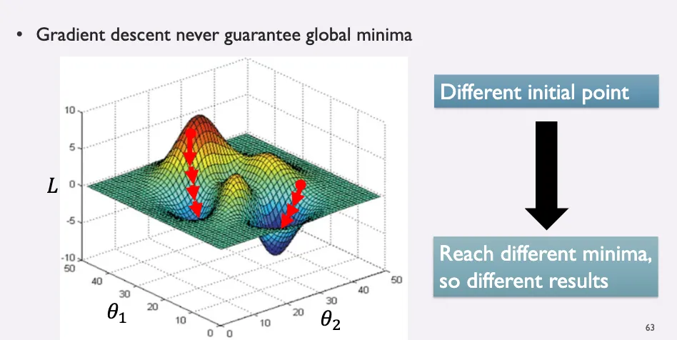
#Gradient Descent

Gradient Descent is the cornerstone optimization algorithm used to minimize the loss function by iteratively adjusting the model's parameters. It plays a pivotal role in training neural networks and other machine learning models.

#How Gradient Descent Works

Initialization:
- Start with an initial guess for the parameters ( \theta ), often initialized randomly or using specific initialization strategies to promote faster convergence.
Compute Gradients:
- Calculate the gradient of the loss function ( L ) with respect to each parameter ( \theta ): $\frac{\partial L}{\partial \theta}$
- The gradient indicates the direction of the steepest ascent in the loss landscape.
Update Parameters:
- Adjust the parameters in the opposite direction of the gradient to minimize the loss: $\theta \leftarrow \theta - \alpha \frac{\partial L}{\partial \theta}$ Where:
  - ( \alpha ) is the learning rate, determining the size of the parameter updates.
  - Choosing an appropriate ( \alpha ) is crucial; too large can cause overshooting, while too small can slow down convergence.
Iterate:
- Repeat the process of computing gradients and updating parameters until convergence criteria are met (e.g., minimal change in loss or a maximum number of iterations).